7.9 KiB
Binary search tree
As shown in the figure below, a binary search tree satisfies the following conditions.
- For the root node, the value of all nodes in the left subtree
<the value of the root node<the value of all nodes in the right subtree. - The left and right subtrees of any node are also binary search trees, i.e., they satisfy condition
1.as well.
Operations on a binary search tree
We encapsulate the binary search tree as a class BinarySearchTree and declare a member variable root pointing to the tree's root node.
Searching for a node
Given a target node value num, one can search according to the properties of the binary search tree. As shown in the figure below, we declare a node cur, start from the binary tree's root node root, and loop to compare the size between the node value cur.val and num.
- If
cur.val < num, it means the target node is incur's right subtree, thus executecur = cur.right. - If
cur.val > num, it means the target node is incur's left subtree, thus executecur = cur.left. - If
cur.val = num, it means the target node is found, exit the loop, and return the node.
The search operation in a binary search tree works on the same principle as the binary search algorithm, eliminating half of the cases in each round. The number of loops is at most the height of the binary tree. When the binary tree is balanced, it uses O(\log n) time. The example code is as follows:
[file]{binary_search_tree}-[class]{binary_search_tree}-[func]{search}
Inserting a node
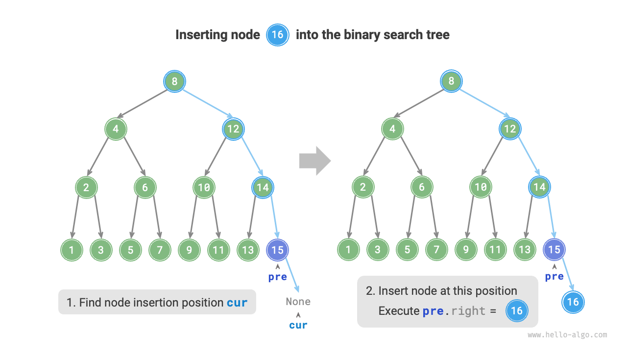
Given an element num to be inserted, to maintain the property of the binary search tree "left subtree < root node < right subtree," the insertion operation proceeds as shown in the figure below.
- Finding insertion position: Similar to the search operation, start from the root node, loop downwards according to the size relationship between the current node value and
num, until the leaf node is passed (traversed toNone), then exit the loop. - Insert the node at this position: Initialize the node
numand place it whereNonewas.
In the code implementation, note the following two points.
- The binary search tree does not allow duplicate nodes to exist; otherwise, its definition would be violated. Therefore, if the node to be inserted already exists in the tree, the insertion is not performed, and the node returns directly.
- To perform the insertion operation, we need to use the node
preto save the node from the previous loop. This way, when traversing toNone, we can get its parent node, thus completing the node insertion operation.
[file]{binary_search_tree}-[class]{binary_search_tree}-[func]{insert}
Similar to searching for a node, inserting a node uses O(\log n) time.
Removing a node
First, find the target node in the binary tree, then remove it. Similar to inserting a node, we need to ensure that after the removal operation is completed, the property of the binary search tree "left subtree < root node < right subtree" is still satisfied. Therefore, based on the number of child nodes of the target node, we divide it into three cases: 0, 1, and 2, and perform the corresponding node removal operations.
As shown in the figure below, when the degree of the node to be removed is 0, it means the node is a leaf node and can be directly removed.
As shown in the figure below, when the degree of the node to be removed is 1, replacing the node to be removed with its child node is sufficient.
When the degree of the node to be removed is 2, we cannot remove it directly, but need to use a node to replace it. To maintain the property of the binary search tree "left subtree < root node < right subtree," this node can be either the smallest node of the right subtree or the largest node of the left subtree.
Assuming we choose the smallest node of the right subtree (the next node in in-order traversal), then the removal operation proceeds as shown in the figure below.
- Find the next node in the "in-order traversal sequence" of the node to be removed, denoted as
tmp. - Replace the value of the node to be removed with
tmp's value, and recursively remove the nodetmpin the tree.
The operation of removing a node also uses O(\log n) time, where finding the node to be removed requires O(\log n) time, and obtaining the in-order traversal successor node requires O(\log n) time. Example code is as follows:
[file]{binary_search_tree}-[class]{binary_search_tree}-[func]{remove}
In-order traversal is ordered
As shown in the figure below, the in-order traversal of a binary tree follows the traversal order of "left \rightarrow root \rightarrow right," and a binary search tree satisfies the size relationship of "left child node < root node < right child node."
This means that when performing in-order traversal in a binary search tree, the next smallest node will always be traversed first, thus leading to an important property: The sequence of in-order traversal in a binary search tree is ascending.
Using the ascending property of in-order traversal, obtaining ordered data in a binary search tree requires only O(n) time, without the need for additional sorting operations, which is very efficient.
Efficiency of binary search trees
Given a set of data, we consider using an array or a binary search tree for storage. Observing the table below, the operations on a binary search tree all have logarithmic time complexity, which is stable and efficient. Arrays are more efficient than binary search trees only in scenarios involving frequent additions and infrequent searches or removals.
Table Efficiency comparison between arrays and search trees
| Unsorted array | Binary search tree | |
|---|---|---|
| Search element | O(n) |
O(\log n) |
| Insert element | O(1) |
O(\log n) |
| Remove element | O(n) |
O(\log n) |
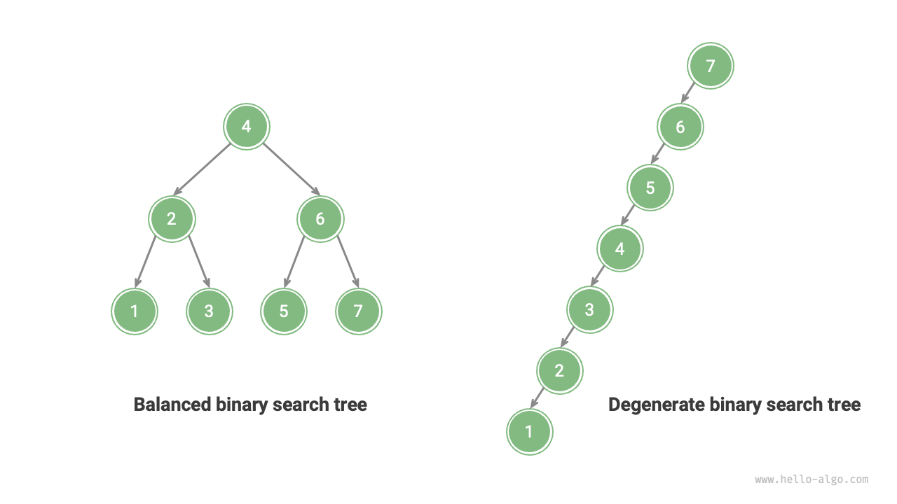
Ideally, the binary search tree is "balanced," allowing any node can be found within \log n loops.
However, if we continuously insert and remove nodes in a binary search tree, it may degenerate into a linked list as shown in the figure below, where the time complexity of various operations also degrades to O(n).
Common applications of binary search trees
- Used as multi-level indexes in systems to implement efficient search, insertion, and removal operations.
- Serves as the underlying data structure for certain search algorithms.
- Used to store data streams to maintain their ordered state.


