6.3 KiB

Raw Blame History

Graph

A "graph" is a type of nonlinear data structure, consisting of "vertices" and "edges". A graph G can be abstractly represented as a collection of a set of vertices V and a set of edges E. The following example shows a graph containing 5 vertices and 7 edges.


\begin{aligned}
V & = \{ 1, 2, 3, 4, 5 \} \newline
E & = \{ (1,2), (1,3), (1,5), (2,3), (2,4), (2,5), (4,5) \} \newline
G & = \{ V, E \} \newline
\end{aligned}

If vertices are viewed as nodes and edges as references (pointers) connecting the nodes, graphs can be seen as a data structure that extends from linked lists. As shown below, compared to linear relationships (linked lists) and divide-and-conquer relationships (trees), network relationships (graphs) are more complex due to their higher degree of freedom.

Common types of graphs

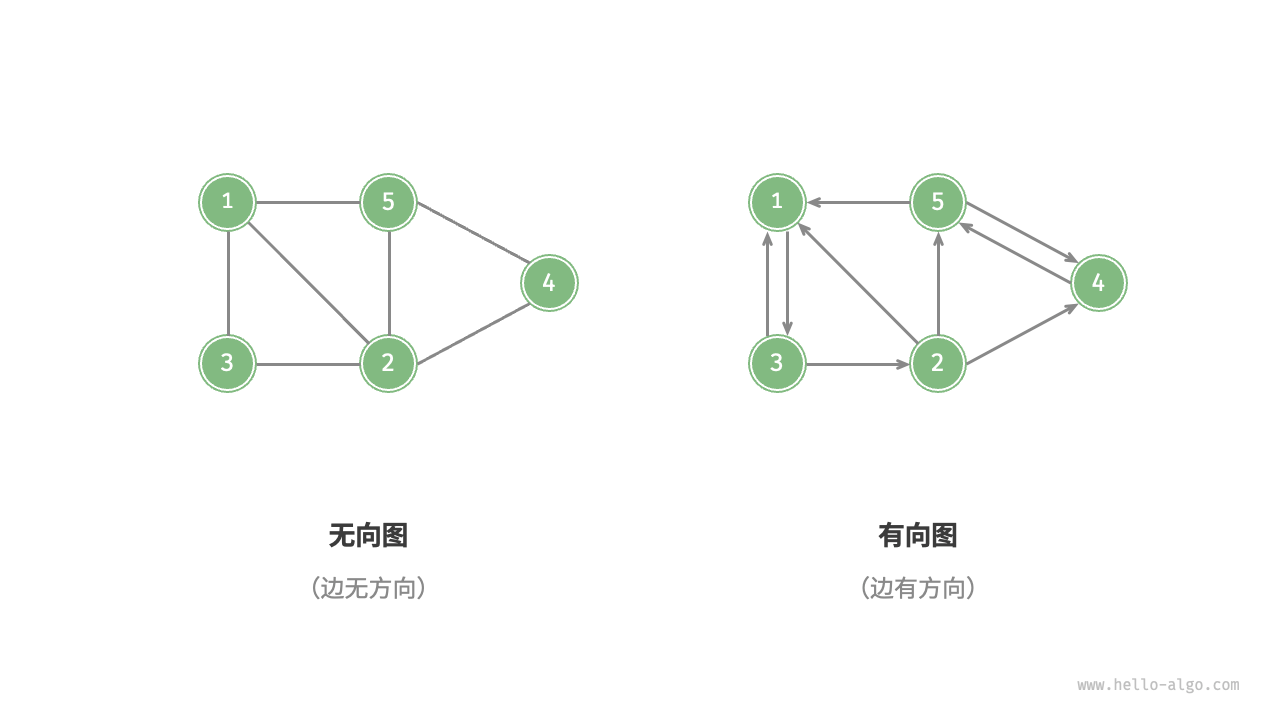
Based on whether edges have direction, graphs can be divided into "undirected graphs" and "directed graphs", as shown below.

In undirected graphs, edges represent a "bidirectional" connection between two vertices, for example, the "friendship" in WeChat or QQ.
In directed graphs, edges have directionality, that is, the edges A \rightarrow B and A \leftarrow B are independent of each other, for example, the "follow" and "be followed" relationship on Weibo or TikTok.

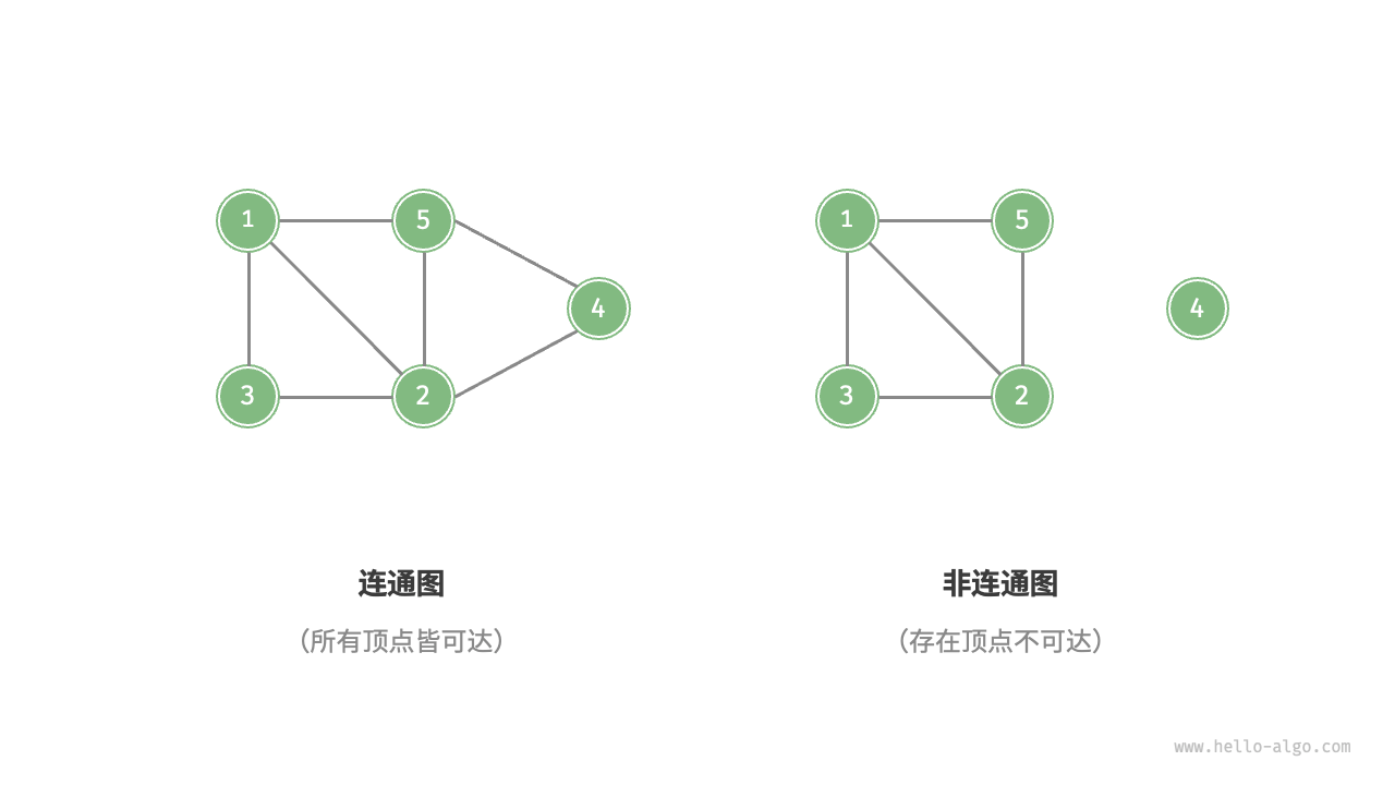
Based on whether all vertices are connected, graphs can be divided into "connected graphs" and "disconnected graphs", as shown below.

For connected graphs, it is possible to reach any other vertex starting from a certain vertex.
For disconnected graphs, there is at least one vertex that cannot be reached from a certain starting vertex.

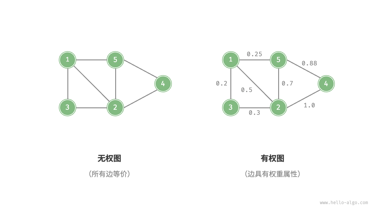
We can also add a "weight" variable to edges, resulting in "weighted graphs" as shown below. For example, in mobile games like "Honor of Kings", the system calculates the "closeness" between players based on shared gaming time, and this closeness network can be represented with a weighted graph.

Graph data structures include the following commonly used terms.

"Adjacency": When there is an edge connecting two vertices, these two vertices are said to be "adjacent". In the above figure, the adjacent vertices of vertex 1 are vertices 2, 3, and 5.
"Path": The sequence of edges passed from vertex A to vertex B is called a "path" from A to B. In the above figure, the edge sequence 1-5-2-4 is a path from vertex 1 to vertex 4.
"Degree": The number of edges a vertex has. For directed graphs, "in-degree" refers to how many edges point to the vertex, and "out-degree" refers to how many edges point out from the vertex.

Representation of graphs

Common representations of graphs include "adjacency matrices" and "adjacency lists". The following examples use undirected graphs.

Adjacency matrix

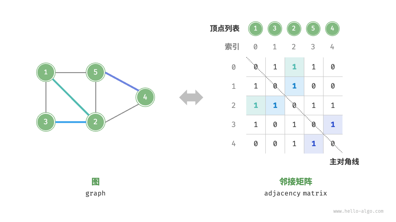
Let the number of vertices in the graph be n, the "adjacency matrix" uses an n \times n matrix to represent the graph, where each row (column) represents a vertex, and the matrix elements represent edges, with 1 or 0 indicating whether there is an edge between two vertices.

As shown below, let the adjacency matrix be M, and the list of vertices be V, then the matrix element M[i, j] = 1 indicates there is an edge between vertex V[i] and vertex V[j], conversely M[i, j] = 0 indicates there is no edge between the two vertices.

Adjacency matrices have the following characteristics.

A vertex cannot be connected to itself, so the elements on the main diagonal of the adjacency matrix are meaningless.
For undirected graphs, edges in both directions are equivalent, thus the adjacency matrix is symmetric about the main diagonal.
By replacing the elements of the adjacency matrix from 1 and 0 to weights, it can represent weighted graphs.

When representing graphs with adjacency matrices, it is possible to directly access matrix elements to obtain edges, thus operations of addition, deletion, lookup, and modification are very efficient, all with a time complexity of O(1). However, the space complexity of the matrix is O(n^2), which consumes more memory.

Adjacency list

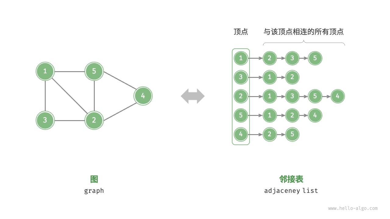
The "adjacency list" uses n linked lists to represent the graph, with each linked list node representing a vertex. The i-th linked list corresponds to vertex i and contains all adjacent vertices (vertices connected to that vertex). The figure below shows an example of a graph stored using an adjacency list.

The adjacency list only stores actual edges, and the total number of edges is often much less than n^2, making it more space-efficient. However, finding edges in the adjacency list requires traversing the linked list, so its time efficiency is not as good as that of the adjacency matrix.

Observing the above figure, the structure of the adjacency list is very similar to the "chaining" in hash tables, hence we can use similar methods to optimize efficiency. For example, when the linked list is long, it can be transformed into an AVL tree or red-black tree, thus optimizing the time efficiency from O(n) to O(\log n); the linked list can also be transformed into a hash table, thus reducing the time complexity to O(1).

Common applications of graphs

As shown in the table below, many real-world systems can be modeled with graphs, and corresponding problems can be reduced to graph computing problems.

Table Common graphs in real life

	Vertices	Edges	Graph Computing Problem
Social Networks	Users	Friendships	Potential Friend Recommendations
Subway Lines	Stations	Connectivity Between Stations	Shortest Route Recommendations
Solar System	Celestial Bodies	Gravitational Forces Between Celestial Bodies	Planetary Orbit Calculations

6.3 KiB Raw Blame History